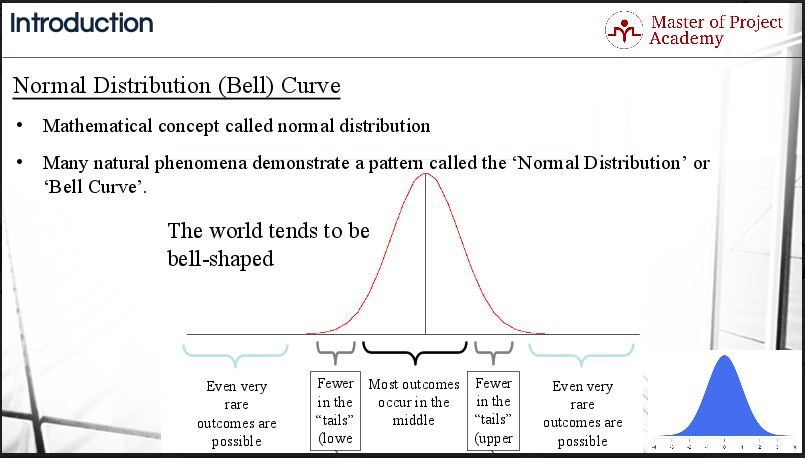
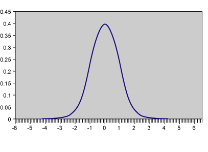
The normal distribution curve is one of the most important statistical concepts in lean six sigma. Understand the role that probability distributions play in determining.

Normal Distribution
Typically in a six sigma project you are using dmaic methodology.

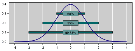
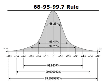
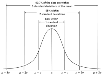
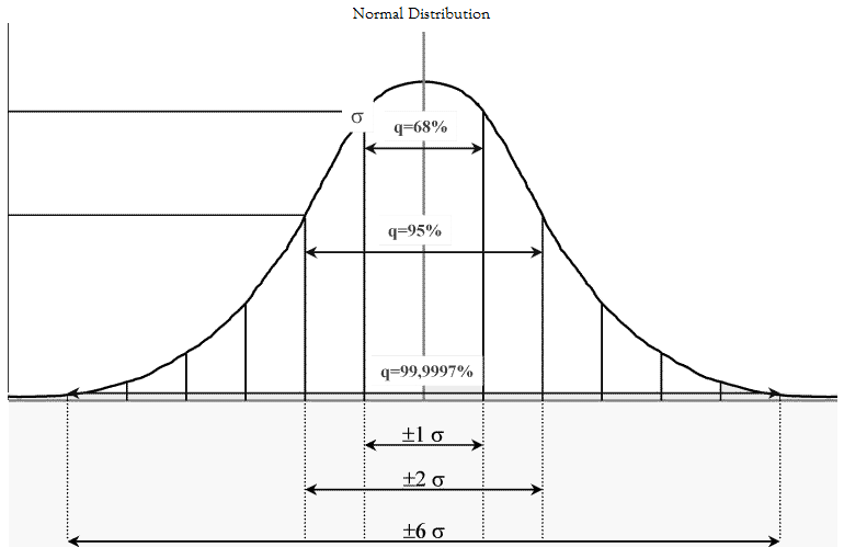
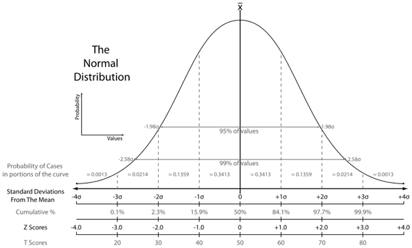
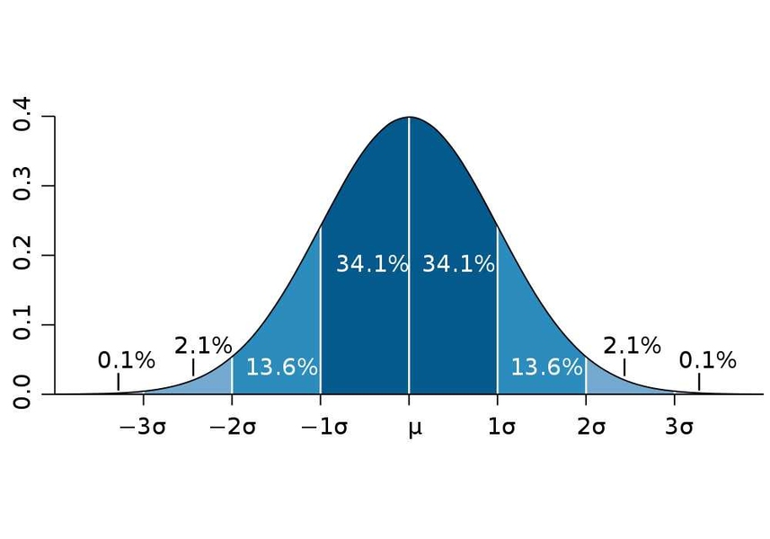
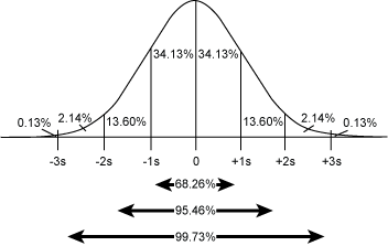
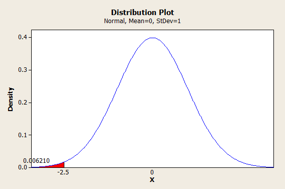
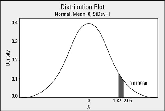
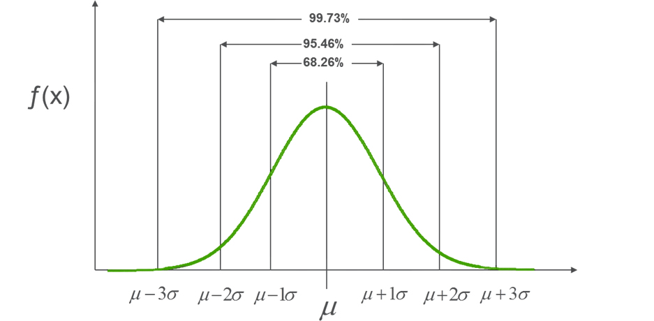
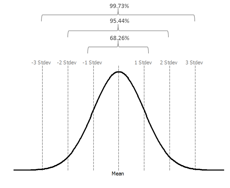
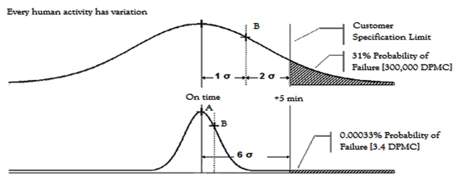
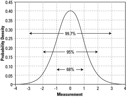
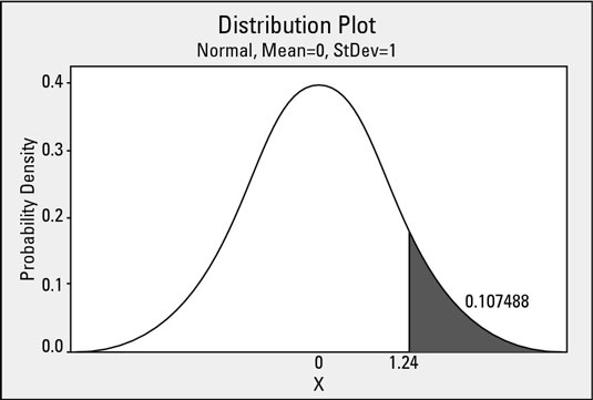
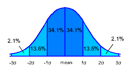
Six sigma probability distribution. Lets say during the define phase you chartered a project to see if you could improve a process that had a binomial outcome. 68 of the distribution area under the curve is about 1 standard deviation from the mean. For example you can easily look up the area under the standard normal curve greater than 124 in the table.
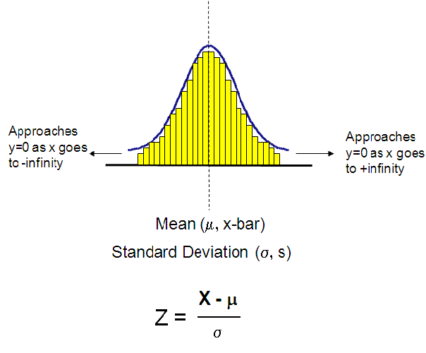
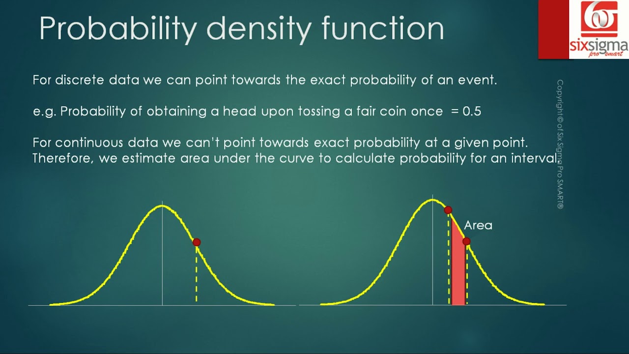
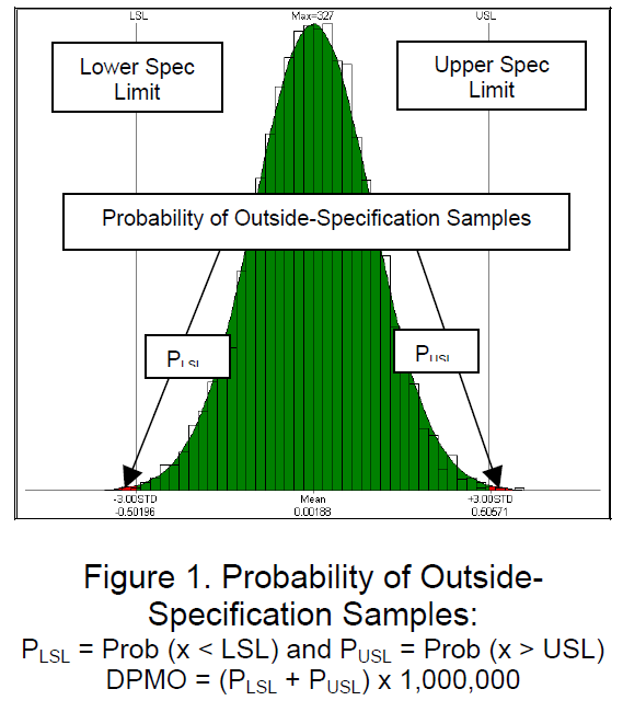
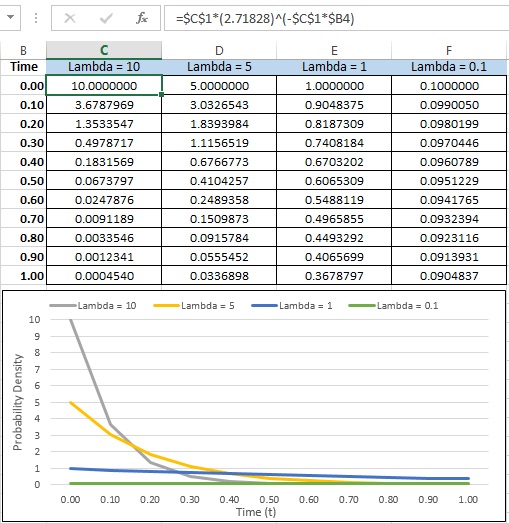
In the statistical tools of six sigma you frequently calculate probabilities using the standard normal table. Where e is a constant of 271828 x is the number of occurrences and l can equate to a sample size multiplied by the probability of occurrence ie npnpx 0 has application as a six sigma metric for yield which equates to y px 0 e l e du e dpu where d is defects u is unit and dpu is defects per unit. Understanding probabilities can provide black belts with the tools to make predictions about events or event combinations.
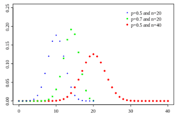
You even might use the binomial distribution to articulate the business case for why you should do the project in the first place for instance event a should be binomial but its clearly not. The normal distribution curve visualizes the variation in a dataset. Lean six sigma solves problems where the number of defects is too high.
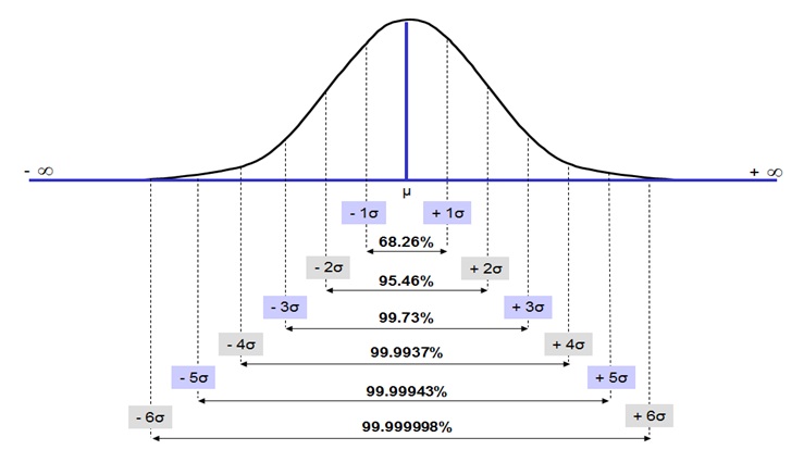
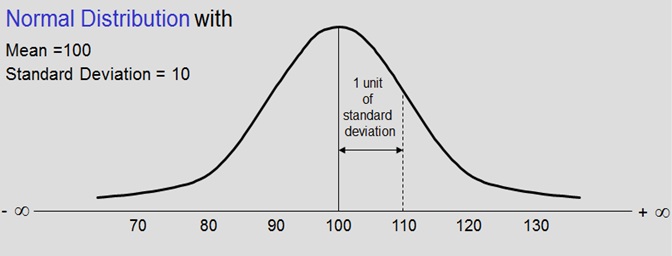
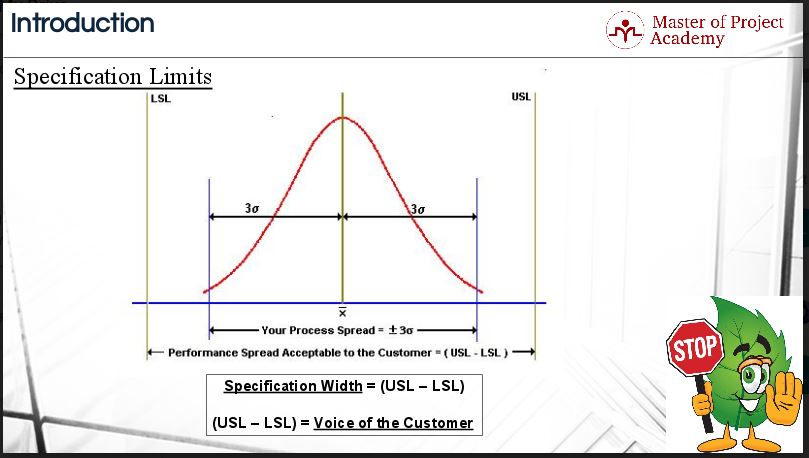
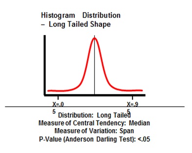
The standard deviation is the square root of the variance and therefore 5. Probability of occurrence sigma value z cum of population 58 65 72 79 86 93 100 107 114 121 128 135 142003 135 2275 1587 500 841 977 9986 99997. This article will expand upon the notion of shape described by the distribution for both the population and sample.
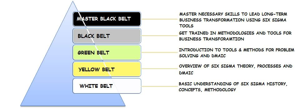
Six sigma green belts receive training focused on shape center and spread. Therefore 35 5 30 is the lower value and 355 40 is the upper value. The probability from the table is 0107488.
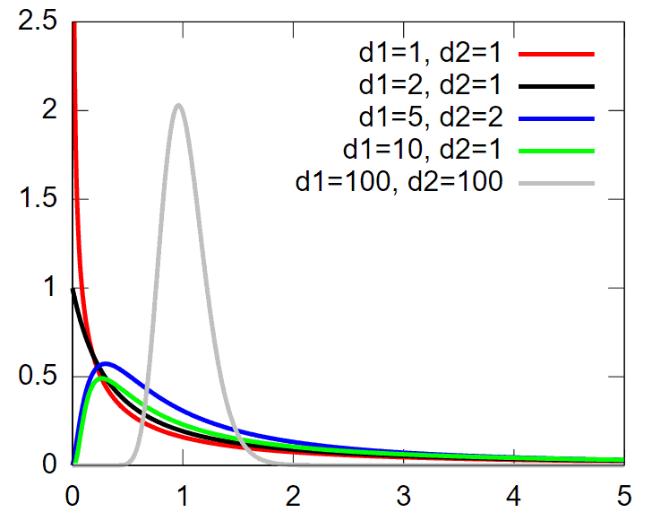
Similarly there are two broad types of probability distribution depending on the data type of the random variable. In a six sigma context it is often important to calculate the likelihood that a combination of events or that an ordered combination of events will occur. The concept of shape however is limited to just the normal distribution for continuous data.
In my previous post on data type for lean six sigma projects opens in new tab we talked about two types of data. Types of probability distribution. Make assumptions given a known distribution.
A high number of defects statistically equals high variation in the process. Example of using binomial probability in a six sigma project.
Understanding Statistical Distributions For Six Sigma
Six Sigma What Is The Normal Distribution Curve
What Is Six Sigma What You Need To Know To Pass Your Certification
Six Sigma Text Png Download 1098 631 Free Transparent Six Sigma Png Download Cleanpng Kisspng
Gaussian Distribution Lean Manufacturing And Six Sigma Definitions
Six Sigma Dmaic Process Measure Phase Measurement System International Six Sigma Institute

Six Sigma Explorescm

Six Sigma Powerpoint Template Powerpoint Templates Powerpoint Professional Powerpoint Presentation
Understanding Process Sigma Level
Normal Distribution
Six Sigma Probability Chart The Future

Six Sigma Wikipedia

Normal Distribution For Lean Six Sigma Lean Six Sigma Simplified
Six Sigma Selling Fear Bullion Directory

What Is Six Sigma Dmaictools Com

Normsinv Function For Microsoft Excel Six Sigma Ninja

Six Sigma Lean Manufacturing And Six Sigma Definitions
Explained Sigma Mit News Massachusetts Institute Of Technology
A Simple Introduction To The Normal Distribution Youtube
What Is Six Sigma What You Need To Know To Pass Your Certification

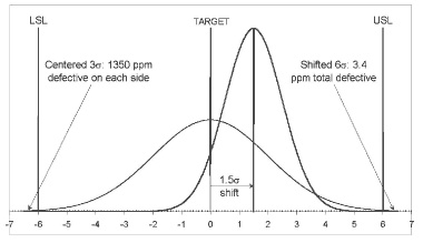
Why Not 4 5 Sigma Dmaictools Com
Six Sigma For Beginner

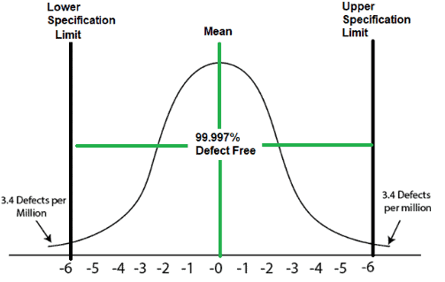
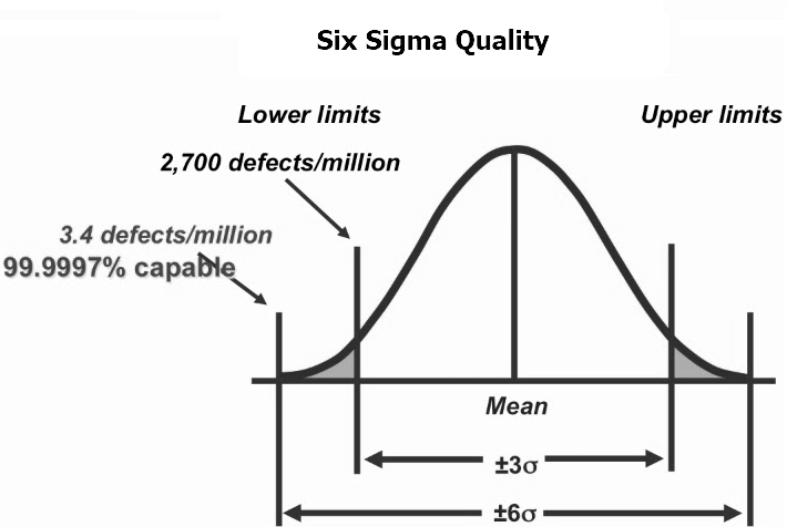
Six Sigma 3 4 Dpmo Why Quality Gurus

1

Pmbok Standard Deviation Formula Is Most Often Wrong Skillpower

Statistical Process Control Calculator Tutorial
What Is Six Sigma Vskills Blog
Six Sigma 3 4 Dpmo Why Quality Gurus

Application Of Statistical Analysis Six Sigma Is Easy Youtube

Six Sigma Events
Hypothesis Testing Fear No More

Six Sigma Basics

Demystifying Six Sigma Metrics In Software Intechopen

Six Sigma 3 4 Dpmo Why Quality Gurus

Statistical Six Sigma Definition
Six Sigma Fad Or Fundamental
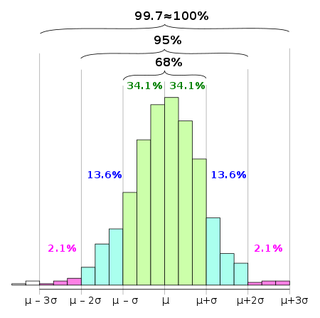
68 95 99 7 Rule Wikipedia

Probability Distribution For Lean Six Sigma Lean Six Sigma Simplified

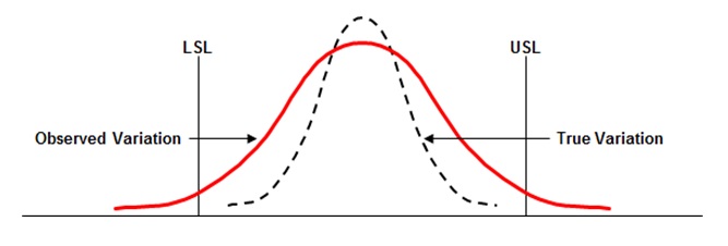
Process Variation And Capability Assessment
Six Sigma Dmaic Process Measure Phase Process Capability International Six Sigma Institute
Why The Binomial Distribution Is Useful For Six Sigma Projects

Six Sigma Lean Manufacturing And Six Sigma Definitions

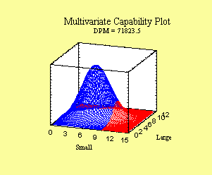
Multivariate Six Sigma

Basics Of Probability Binomial Poisson Distribution Illustration With Practical Examples Youtube
Six Sigma For Beginner

Normal Distribution For Lean Six Sigma Lean Six Sigma Simplified
Statistical Process Control Spc Tutorial
Why The Binomial Distribution Is Useful For Six Sigma Projects

1
Data Distributions What You Need To Know For A Six Sigma Certification Exam
6 Sigma Calculator To Convert Between Ppm Dpmo Sigma Trending Sideways

Types Of Distributions In Six Sigma
Six Sigma Dmaic Process Measure Phase Measurement System International Six Sigma Institute

What Is Six Sigma Dmaictools Com

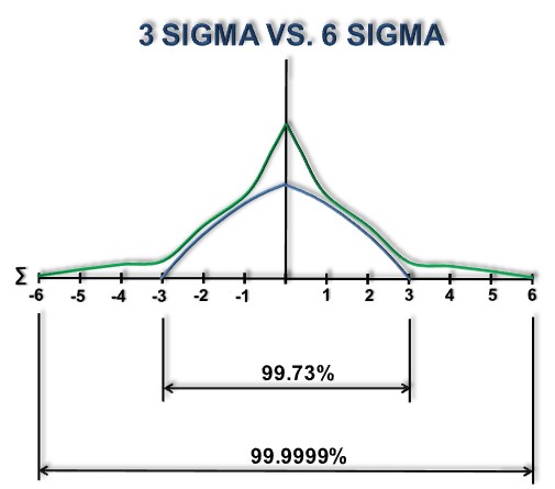
Three Sigma Vs Six Sigma
How To Analyze Normal Variation And Probability For Six Sigma Dummies

Process Variation And Capability Assessment
Six Sigma What Is The Normal Distribution Curve
How To Analyze Normal Variation And Probability For Six Sigma Dummies

Calculating Sigma Levels In Excel Six Sigma Ninja
Data Distributions What You Need To Know For A Six Sigma Certification Exam

Cpk
How Do The Six Sigma Statistics Work

An Introduction To Excel S Normal Distribution Functions Exceluser Com
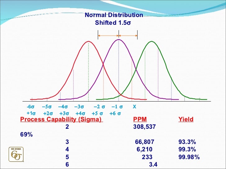
Understanding Process Capability And Sigma Shift

Normal Distribution Table 2 Normal Distribution Process Capability Sigma
Data Distributions What You Need To Know For A Six Sigma Certification Exam
Normal Distribution And Normality Lean Sigma Corporation

Explaining Six Sigma Presentation Diagrams Ppt Template With 6s Principles Concepts And Dmaic Process Powerpoint Charts
Understanding Statistical Distributions For Six Sigma

Z Value Statistics For Six Sigma Made Easy Book

Six Sigma Wikipedia
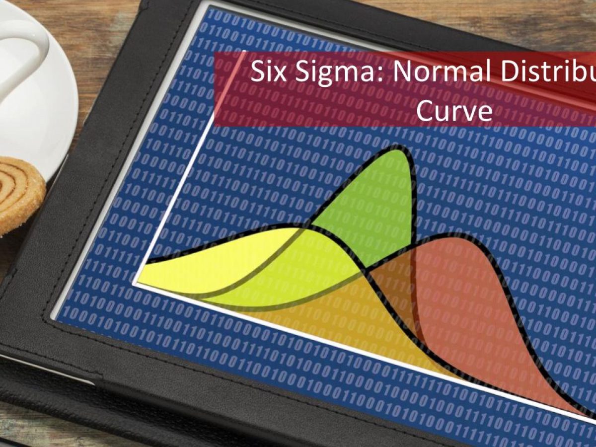
Six Sigma What Is The Normal Distribution Curve

1

Six Sigma Simply Explained
Lean Six Sigma Intechopen
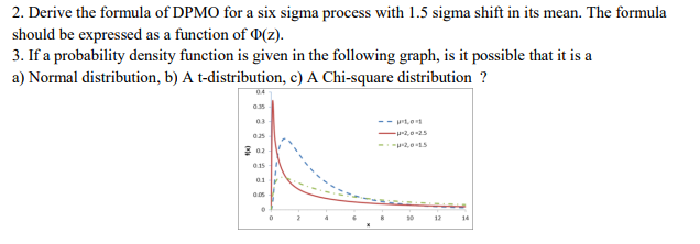
Solved 2 Derive The Formula Of Dpmo For A Six Sigma Proc Chegg Com

Normal Distribution Normal Distribution Statistics Math Standard Deviation

Basic Statistics
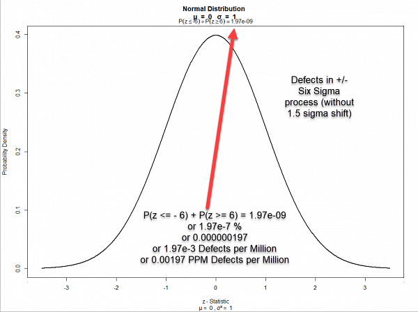
Z 6 Probability And The Standard Normal Distribution Westgard
Chapter 14 Limited Mathematical Background For Design For Six Sigma Dfss Six Sigma And Beyond Design For Six Sigma Volume Vi

Probability Distribution For Lean Six Sigma Lean Six Sigma Simplified

Six Sigma Process With R Analyzing Process Capabilities By Roberto Salazar The Startup Medium

Figure 2 From Robust Design Optimization Of Pm Smc Motors For Six Sigma Quality Manufacturing Semantic Scholar
Six Sigma Dmaic Process Measure Phase Measurement System International Six Sigma Institute
High Sigma Events They Re Not All Black Swans Six Figure Investing

Commonly Used Distribution In Six Sigma Iso Consultant In Kuwait
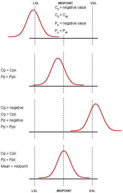
Cpk
How To Analyze Normal Variation And Probability For Six Sigma Dummies
Risk For Six Sigma Quality Analysis Software Using Monte Carlo Simulation Palisade
Everything You Need To Know About What Is Six Sigma Updated
Defects Per Million Opportunities Dpmo And Z Scores Diving Into The Six Sigma Rabbit Hole

Different Types Of Probability Distribution Characteristics Examples Data Science Learning Data Science Statistics Statistics Math

Six Sigma Method And Its Applications In Project Management
Understanding The Normal Distribution With Python By Tony Yiu Towards Data Science
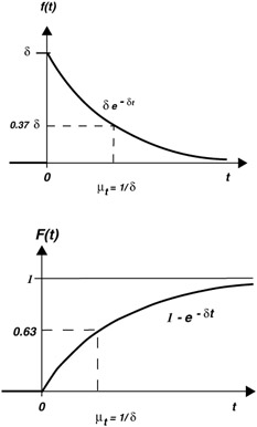
Exponential Distribution
Data Distributions What You Need To Know For A Six Sigma Certification Exam
How To Analyze Normal Variation And Probability For Six Sigma Dummies

Https Encrypted Tbn0 Gstatic Com Images Q Tbn And9gct9ujlz3opp Ivkhsmbzg8kjeufjwh0yh Osisnr Tg5qulmgs Usqp Cau

Amazon Com Probability Distributions Six Sigma Thinking 9781393113584 Savant Sumeet Savant Sumeet Books

Probability Distributions Ebook By Sumeet Savant 9781393113584 Rakuten Kobo Greece
Understanding Statistical Distributions For Six Sigma
Six Sigma Dmaic Process Measure Phase Measurement System International Six Sigma Institute


Post a Comment for "Six Sigma Probability Distribution"